# Convolutional Neural Networks

# Introduction

Convolutional Neural Networks (CNNs) are similar to the Neural Networks covered in the previous sections. They comprise neurons with learnable weights and biases, where every neuron receives an initial value (input), calculates a function (dot product) and optionally follows it with a nonlinearity (LeCun et al., 1999). The network still expresses a single score function that has for argument the raw image pixels (input) and for value the class scores (output), and it still has a loss function on the last fully connected layer (e.g. Softmax).

Differently from classic NNs, CNNs include a number of convolutional layers and optional pooling layers, explained in more detail below.

CNNs represent an interesting evolution in the computer vision field: they perform extremely well on images and videos since the convolutional layers contained in the architecture can exploit the spatial feature locality of images. The intuition behind this is that the pixels contained in a region of an image are more likely to be related than pixels far away from each other.

According to this concept, the convolution operation acts on groups of adjacent pixels, which gives the advantage of drastically reducing the complexity of the model. This concept is also known as "local connectivity". This leads to faster training; reduces the chance of overfitting, since fewer parameters are used; and allows to scale to larger images, since less memory is required.

Moreover, the network can include a number of pooling layers to progressively downscale the input. This effectively reduces the number of parameters required to process an image, which decreases the total computation time as well as helping to control overfitting.

# The First CNNs

Research on the brain of cats carried out by Hubel & Wiesel (1962) introduced a new model for how these animals visually perceive the world: they demonstrated that a cat’s visual cortex includes neurons that exclusively respond to other neurons in their direct environment.

In their paper, they describe two basic cell types: simple and complex cells. Simple cells respond to specific edge-like patterns within their narrow receptive field; they identify basic shapes, such as lines in a fixed area and at a specific angle. Complex cells have larger receptive fields, which means they can capture details at a higher level of detail. Also, they are locally invariant to the exact position of the pattern.

The first artificial neural network based on the model described by Hubel & Wiesel was proposed by Fukushima & Miyake in 1982. Their hierarchical multilayered neural network, named "Neocognitron", was based on the idea of simple and complex cells: the simple cells basically perform a convolution, while the complex cells perform average pooling. Due to mainly slow performance, the lack of a real application, and the lack of a community of researchers promoting it, this network did not attract much attention at that time.

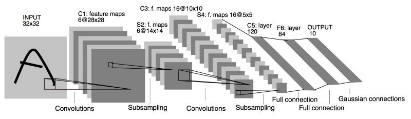
The first set of CNNs to be used in production were developed by LeCun et al. (1999), who started to work on this technology since 1989 and reached the highest success with the publication of their paper "Object recognition with gradient-based learning". The refined model described in this last paper was commercially employed to recognise hand-written characters in zip codes. Their model is shown in the Figure 1.

# Architecture Overview

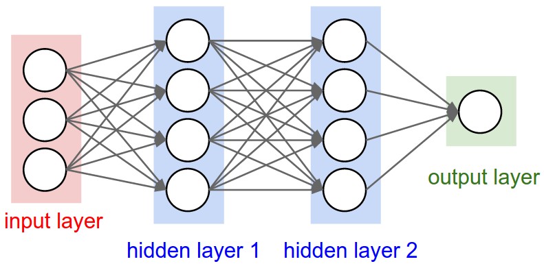
As described in the introductory section, Convolutional Neural Networks are more suited than NN to perform, for example, classification tasks on images and videos (LeCun et al., 1999). Unlike a traditional neural network, a CNN contains neurons arranged in the 3 dimensions width, height and depth. Each neuron in a layer is only connected to a small region of the layer that precedes it, as opposed to being connected to all of the previous layer’s neurons (i.e. neurons are locally-connected instead of fully-connected). Nevertheless, the final layers of a CNN architecture reduce a full image into a single vector of class scores, arranged along the depth dimension. Figure 2 shows an architectural comparison between a NN and a CNN.

# Layers of a CNN

A simple CNN is composed of a sequence of layers that transform one volume of activations to another through a nonlinear function. The three main types of layer used to build a CNN are the Convolutional, Pooling and Fully Connected layers (LeCun et al., 1999).

An example CNN architecture that translates an image into class scores has a layer structure of type [INPUT -> CONV -> RELU -> POOL -> FC]. Each layer’s operation is briefly described below:

• The INPUT layer holds the raw image pixel values and is represented, for example, by the vector [224x224x3]. It has three dimensions: width and height equal to 224 (which correspond to the image’s width and height), and depth 3 (e.g. for an RGB image).

• The CONV layer computes the output of the neurons that are connected to local regions in the input. Each neuron computes the dot product between its weights and a small region of the input they are connected to. If 12 filters were used in this layer, the resulting volume would be [224x224x12].

• The RELU layer applies an element-wise activation function, in this case , which sets the output value of each neuron. The output is then used as input for the next layer’s neurons.

• The POOL layer (usually max pooling) downsamples the spatial dimensions of the previous layer’s output by a factor of 2, resulting in a volume such as [112x112x12]. The depth is not affected by this operation.

• The FC (fully-connected) layer computes the class scores, resulting in a volume of, for example, [1x1x10]. The depth value at the last layer corresponds to the number of categories for which a score is computed. Every neuron in this layer is connected to all the neurons in the previous layer.

Thanks to the basic architecture outlined, a CNN is able to transform the original image (pixel values) to the final class scores. To note is that the RELU and POOL layers implement a fixed function, whereas the CONV and FC layers implement a function not only affected by the activations in the input volume but also by weights and biases. These parameters are still trained with gradient descent.

In the next sections, the layers that characterise a CNN are analysed in greater detail.

# Convolutional Layer

The convolutional layer uses filters (also known as kernels) to detect the features present in an image. A filter is simply a matrix of values that can detect specific features, such as horizontal or vertical edges. Filters are spatially small (small width and height, generally 3x3 or 5x5) and have always the same depth of the input volume (e.g. depth 3 for RGB or 1 for grayscale images).

Every filter is convolved across the width and height of the input volume: this computes the dot product between the values of the filter and the values of the input at any position. Starting from the top left, the filter slides over the width and height of the input volume; for each convolution operation, this produces a 2D activation map that holds the response of that filter at any spatial position (see Figure 3).

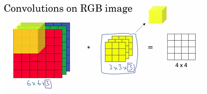
Every convolutional layer can contain a number of 3D filters (yellow cube shown in Fig. 3), each producing a separate 2D activation map. In this case, the output is a volume composed by all the resulting activation maps stacked along the depth dimension. For instance, if 12 filters of size 3x3x3 are contained in a convolutional layer, the output volume will have depth equal to 12.

The filters in the first layers of a CNN activate when they see basic visual features (e.g. horizontal and vertical edges) while the filters in deeper layers of the network capture more complex visual feature (e.g. honeycomb or circular shapes).

# Local Connectivity

Since images have a high-dimensionality, it is often unfeasible to connect each neuron to all neurons in the previous volume (which is what happens in the layers of a fully connected NN). In contrast, the convolutional layer tries to emulate the response of individual neurons to visual stimuli as per the model described by Hubel & Wiesel (1962). In fact, each value in the convolution output volume can be thought of as the output of a neuron that looks only at a small region in the input (i.e. its receptive field). The spatial extent of the observed region is equal to the filter size.

For example, for an input volume with size [32x32x3] and a receptive field 5x5, each neuron in the CNN has weights to a [5x5x3] region in the input volume for a total of 5*5*3 = 75 weights, plus a bias parameter.

# Spatial Arrangement

The hyper-parameters that control the size of the output volume are the depth, the stride and the padding. These are explained below:

• Depth. It corresponds to the number of filters that are applied to an input volume. Each of these filter can look for different patterns in the input volume (e.g. vertical, horizontal, 45 degree edges etc.).

• Stride. It specifies the number of pixels the filter must shift by (i.e. step size). For example, if the stride is 1, the filter moves 1 pixel at a time. If stride is used, a spatially smaller output volume is produced. The minimum stride is 1 and is implied if none is specified, however, a stride of 2 is also commonly used, while higher stride values are rarer.

• Padding. It specifies the number of pixels added to the edges of an image along its spatial dimensions (width and height). It is often referred to as zero-padding, because the added pixels commonly have a value of 0. Padding allows to control the spatial size of an output volume, and can thus preserve an input volume’s width and height. This prevents information from the edges of the input volume to be thrown away during the convolution operation and makes sure that the filter and stride size will fit in the input.

The spatial size of the output volume can be computed as a function of the input volume size (supposing the same width and height), the filter size , the stride (or step size), and the padding with the following formula:

# Parameter Sharing

Convolutional layers use parameter sharing to drastically reduce the number of parameters (Standford University, 2017). The introduction of parameter sharing arises from the assumption that if one feature is useful to compute at a spatial position , then it should be useful also at a different position . Indicating with "depth slice" each volume’s 2D slice of depth (e.g. a volume with depth 96 has 96 depth slices), all neurons in the same depth slice are constrained to use the same weights and bias.

Since all neurons in a single depth slice use the same weight vector, the forward pass of the convolutional layer can be computed, for each depth slice, as a convolution of the neuron’s weights with the input volume. Because of this, sets of weights are commonly referred to as a "filter" or a "kernel", that are convolved with the input. The result of each of these convolutions is an activation map; sets of activation maps are stacked together along the depth dimension to produce the output volume.

Parameter sharing might not always be suitable. If the features to be learnt must be located at a specific location in the image (e.g. nose is always at the centre on a face), it is common to ease the parameter sharing scheme and instead simply call the layer a "locally connected layer".

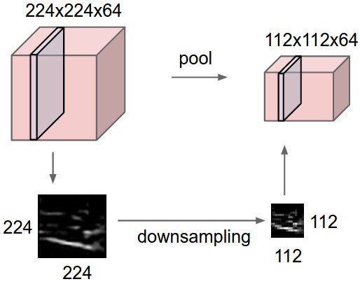
# Pooling Layer

The function of the pooling layer is to progressively reduce the spacial dimensions of the representation (the previous layer’s output volume). This reduces the number of parameters in the network and the total computation that it has to carry out, which helps to control overfitting.

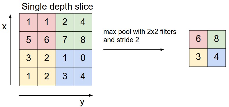
The pooling layer resizes every depth slice of the input volume independently from the others. The most common form of pooling is called max pooling: this uses the MAX operation to only take the maximum input from a fixed region of a depth slice (see Figure 4). The max pooling layer most commonly uses filters of size 2x2 with a stride of 2 along both width and height, which allows to remove the 75% of the activations (i.e. the MAX operator takes in 4 values and returns 1). The depth remains unchanged.

More formally, the pooling layer:

• Has for input a volume of size x x .

• Requires two hyper-parameters:

  • the spatial extent ,

  • the stride .

• Produces a volume of size x x where:

• Is a fixed function of the input, therefore, it does not add parameters to the network.

In practice, only two variations of the max pooling layer are used: the most common is the pooling layer with values ; second to this, values are used (overlapping pooling). Pooling layers with larger receptive field sizes destroy too much information.

Other forms of pooling, such as average pooling or L2-norm pooling, were used in the past. Max pooling, however, was shown to provide better results in practical applications [Boureau et al. (2010) and Boureau et al. (2011)].

Although pooling layers have long been employed in CNNs, recent developments such as the ones proposed by Springenberg et al. (2014) in their paper "Striving for simplicity: The all convolutional net", suggest these could be omitted in favour of a larger stride in some of the network’s convolutional layers. They state that pooling operations do not always improve the performance of CNNs, especially if the network is large enough for the dataset it is being trained on and can learn all the necessary invariances with convolutional layers only. Compared to the state of the art, their network model was able to match the performance or slightly outperform other CNNs on datasets like CIFAR-10 and CIFAR-100 (Krizhevsky & Hinton, 2009).

# Final Considerations

CNNs have proved extremely successful for a variety of tasks, such as face recognition (Schroff et al., 2015), document analysis (Simard et al., 2003), modelling sentences (Kalchbrenner et al., 2014) and many more.

Despite their success, there are numerous challenges that still need to be overcome when using CNNs. One of the biggest challenges regards the substantial amount of training data that they require, which is expensive, labour-intensive and time consuming to obtain. Relatedly, CNNs generally break down if only a few labelled examples are available.

Recongising objects using only a few labelled examples is known as one or few-shot learning. The next section describes this problem in greater detail.

# References

- LeCun, Y., Haffner, P., Bottou, L., & Bengio, Y. (1999). Object recognition with gradient-based learning. In Shape, contour and grouping in computer vision (pp. 319–345). Springer.
- Hubel, D. H., & Wiesel, T. N. (1962). Receptive fields, binocular interaction and functional architecture in the cat’s visual cortex. The Journal of Physiology, 160(1), 106–154.
- Fukushima, K., & Miyake, S. (1982). Neocognitron: A self-organizing neural network model for a mechanism of visual pattern recognition. In Competition and cooperation in neural nets (pp. 267–285). Springer.
- LeCun, Y., Bottou, L., Bengio, Y., & Haffner, P. (1998). Gradient-based learning applied to document recognition. Proceedings of the IEEE, 86(11), 2278–2324.
- Standford University. (2017). Stanford university cs231n: Convolutional neural networks for visual recognition. CNN Notes.
- deeplearning.ai. (2019). Convolutional neural networks.
- Boureau, Y.-L., Ponce, J., & LeCun, Y. (2010). A theoretical analysis of feature pooling in visual recognition. Proceedings of the 27th international conference on machine learning (icml-10), 111–118.
- Boureau, Y.-L., Le Roux, N., Bach, F., Ponce, J., & LeCun, Y. (2011). Ask the locals: Multi-way local pooling for image recognition. Computer vision (iccv), 2011 ieee international conference on, 2651–2658. IEEE.
- Springenberg, J. T., Dosovitskiy, A., Brox, T., & Riedmiller, M. (2014). Striving for simplicity: The all convolutional net. arXiv Preprint arXiv:1412.6806.
- Krizhevsky, A., & Hinton, G. (2009). Learning multiple layers of features from tiny images. Citeseer.
- Schroff, F., Kalenichenko, D., & Philbin, J. (2015). Facenet: A unified embedding for face recognition and clustering. Proceedings of the ieee conference on computer vision and pattern recognition, 815–823.
- Simard, P. Y., Steinkraus, D., & Platt, J. C. (2003). Best practices for convolutional neural networks applied to visual document analysis.
- IEEE.
- Kalchbrenner, N., Grefenstette, E., & Blunsom, P. (2014). A convolutional neural network for modelling sentences. arXiv Preprint arXiv:1404.2188.