Neural Networks
Introduction
Neural Network is a broad term used to describe a vast collection of computational models vaguely inspired by the biological neurons and the connections among them (synapses; Haykin, 1994).
Similarly to the brain, NN are parallel information-processing systems that can build up their own functioning rules over time through "experience", thanks to which they can reorganise their structural constituents, the neurons, to perform tasks such as pattern recognition, motor control, auditory signal-processing and so on.
Haykin (1994, p. 2) provides a more formal definition of Neural Network, describing it as:
"A massively parallel distributed processor made up of simple processing units [neurons], which has a natural propensity for storing experiential knowledge and making it available for use".
This model resembles the human brain in two respects:
Knowledge is acquired from the environment through a learning process.
Synaptic weights are used to store the acquired knowledge.
Gaining experience and learning, in the context of NNs, refer to a particular technique named backpropagation, for the first time applied to this field by Paul Werbos in 1974. Backpropagation and the working principles of artificial neurons are discussed in more detail further on.
An example of a feed-forward neural network is illustrated below in Figure 1, along with a basic explanation.
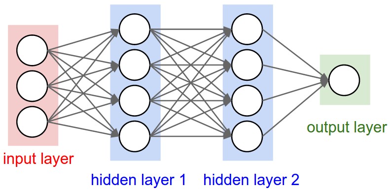
The network receives an input (a single vector), transforms it through a series of hidden layers, and outputs a result. The hidden layers compute nonlinearities that are finally passed to the last fully connected layer in the network (the “output layer”). In classification settings, the neurons in the output layer commonly represent the different categories. Image source: Standford University (2017).
Advantages of Neural Networks
Neural networks offer a number of advantages that make them the most suitable choice for solving certain tasks (Haykin, 1994). Some of the key advantages are listed below:
Generalisation. It is the ability to handle unseen data. After learning from initial input (i.e. training set), NNs can infer relationships on unseen data (i.e. the model can generalise to unseen images). Poor generalisation is achieved when the model maps the training data too closely (overfitting) or when it is not complex enough to accurately capture relationships in the data (underfitting).
Nonlinearity. NNs have the ability to implicitly detect complex, nonlinear relationships between dependent and independent variables. In contrast, linear equations are easier to solve but do not have the same power to learn complex functional mappings.
Parallel Operation. NNs computations can be carried out in parallel and are in some cases best fit for real time applications (e.g. real time object detection). Special hardware devices, such as GPUs, are being designed and manufactured to take advantage of this capability.
Fault Tolerance. The absence of data in one place does not prevent the network from functioning. Inherent fault tolerance ensures that even with major network damage, some of the network capabilities are retained.
While the many advantages of neural networks make them highly employed today, some of their working principles are not fully understood yet. This constitutes one of their best known disadvantages: while they can approximate any function, analysing the weights, biases and network structure does not provide any insights on the structure of the function being approximated. In essence, one cannot be sure of why a NN produced a certain output.
History of Neural Networks
The history of neural networks dates back to 1943, when neurophysiologist Warren McCulloch and mathematician Walter Pitts wrote a paper on how neurons might work, and modelled a simple neural network with electrical circuits (McCulloch & Pitts, 1943). Later, in 1958, Frank Rosenblatt conceived the Perceptron while studying the decision making systems present in the eye of a fly (Rosenblatt, 1958). This is a simplified mathematical model of how a neuron operates and is the oldest neural network still in use today. More on the structure of a neuron can be found below.
Despite some later successes of neural networks, research in the field halted for a number of years. The first major extension of the feedforward neural network appeared in 1971, when Werbos used backpropagation to train a NN, a technique that he later described in his PhD thesis (Werbos, 1974). His findings did not receive attention until rediscovered by Parker (1985) and Rumelhart et al. (1985) which, thanks to the clear framework used to present their ideas, made it widely known within the research community and brought a new wave of interest in the field. Their papers addressed many of the problems that had previously discouraged the research community; as such, from 1986 it was clear how multilayer NNs could be trained to tackle complex learning problems.
Since then, a vast number of NN architectures have been developed and used in fields such as Natural Language Processing, Object and Speech Recognition, Stock Market Analysis, Signal Processing and more. Recently, the increase of available computing power offered by GPUs, the introduction of distributed computing and the rise of Big Data drove the advent of deep learning, a subfield of machine learning most often associated to deep artificial neural networks (i.e. networks with 3 or more hidden layers).
In conclusion, NNs have evolved significantly in the 76 years elapsed since the first attempt at modelling an artificial neuron. Although periods of reduced funding and popularity have marked their history, in the last decade they received extreme interest from the research community, and the upward trend is not thought to end soon.
The Neuron
In nature, a typical neuron consists of a cell body (soma), an axon and a number of dendrites (Haykin, 1994). A neuron receives electrochemical inputs from other neurons at the dendrites level; if the sum of these electrical inputs is sufficiently powerful (i.e. if it surpasses a certain threshold), the neuron activates and transmits an electrochemical signal along the axon. This signal is passed to other neurons through the axon terminals, which are attached to other neurons’ dendrites. These attached neurons may then activate in their turn.
Fundamentally, each neuron performs a weighted sum of its inputs and fires a binary signal if this sum exceeds a certain threshold. From a very large number of simple processing units, the brain is able to perform extremely complex tasks. Figure 2 illustrates a natural neuron in juxtaposition with its artificial counterpart.
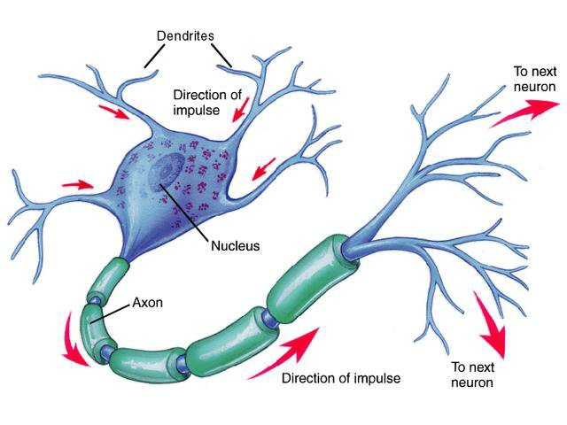
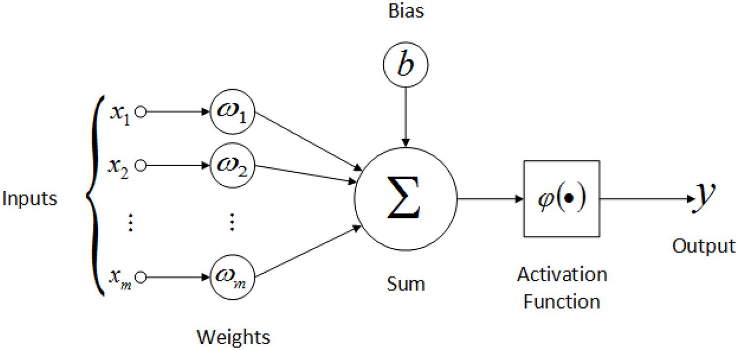
Similar to a biological neuron which receives signals at the dendrites, processes them through the cell body, and sends signals out to other neurons via the axon terminals, the artificial neuron has a number of input channels, a processing stage, and an output that can be sent to multiple other artificial neurons. Left image source: Nazrul et al. (2014).
Artificial neurons are mathematical functions inspired by the biological neuron model. Similarly to a real neuron that receives electrical signals with variable strength, an artificial neuron multiplies each input value by a parameter known as "weight". The weight can be thought of as the strength of the connection between two neurons.
A biological neuron fires an output signal only when the total strength of the input signals exceeds a certain threshold. In an artificial neuron, the total strength of the input signals is represented by the weighted sum of the inputs plus a user defined bias. A nonlinear function known as "activation function" uses this sum to compute the output value of the neuron.
To modify the inter-neuron connection strengths (weights) in order to "learn" and reach a desired design objective, the backpropagation algorithm is used. More on the full learning process of an artificial neural network is covered in further on.
As a final note, it must be said that although artificial NNs are inspired by the neurons and networks in the brain, the implementation of these concepts has diverged significantly from how the brain works. Practically, artificial NNs are approximate and over-simplified models of real brains. Despite this, they have proved extremely effective at solving problems that are difficult to solve for conventional computer architectures. For example, as demonstrated by He et al. (2015), deep NNs have successfully exceeded the reported human level performance on fine-grained recognition (e.g. recognise the 120 species of dogs in the Imagenet dataset, which is non-trivial for humans).
Activation Functions
Activation functions are a crucial component of artificial neural
networks since they introduce nonlinearity, which allows to learn from
complicated, nonlinear mappings between inputs and response variables
(Haykin, 1994, pp. 141–144). In the neuron, an activation function maps
the weighted sum of inputs (plus a bias) to a value in a desired range,
depending on the function chosen (example ranges are
In essence, considering the weighted sum of inputs
where
Types of Activation Function
Many different activation functions exist, however, only a handful of them are used in practice today. The most popular ones are described below.
Sigmoid
This nonlinear function is preferred over the unit step function (or
Heaviside step function) in that it can squash an input to any value
between
Although used historically, the sigmoid function is today rarely employed, mainly due to its related "vanishing gradient" problem, which particularly affects deep networks: essentially, the shape of the sigmoid derivative causes the magnitude of the gradient to shrink exponentially as the network backpropagates the error (see Figure 3). The same problem affects the tanh activation function, which was historically proposed as an improvement over sigmoid.
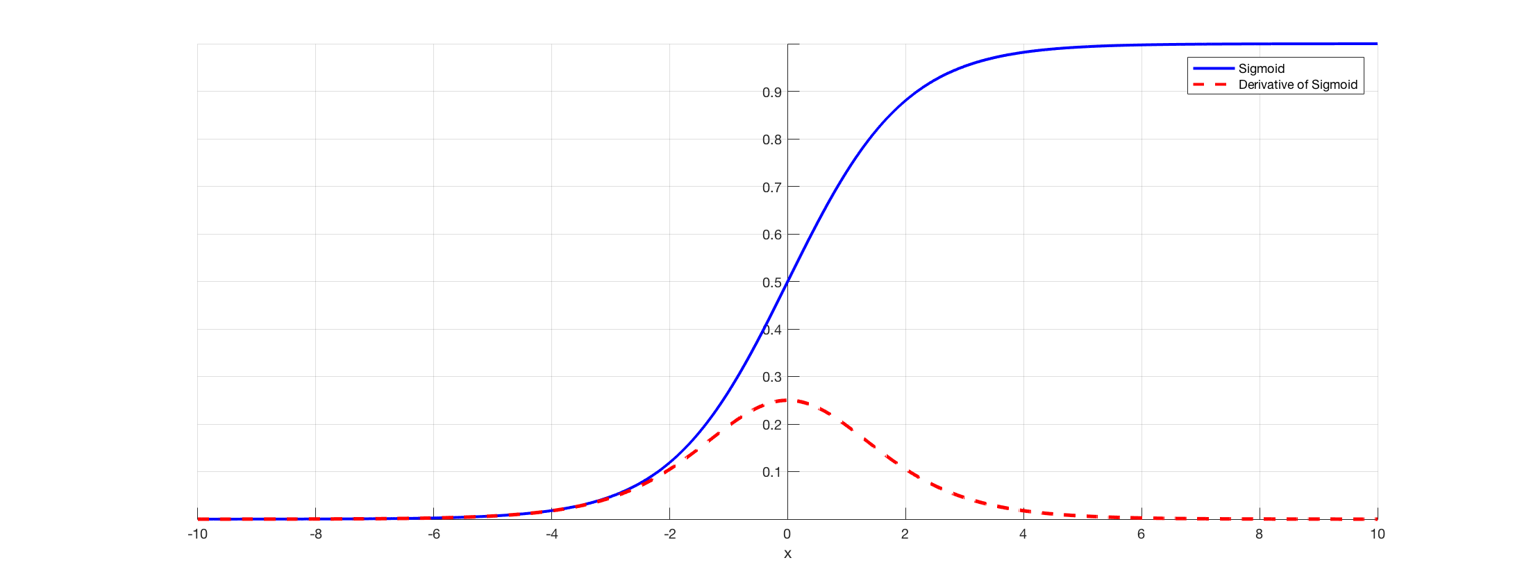
As shown, sigmoid’s derivative cannot have a value higher than 0.25. Moreover, if the output of the sigmoid function is too high or too low (i.e. if it approaches 0 or 1), the derivative becomes much less than 0.25.
This causes the gradient to shrink exponentially as backpropagation works towards the early layers, resulting in a gradient close to 0 at the first layers (vanishing gradient). This is a key problem as it causes the network to stop or slow down learning. Image source: Changhau (2017).
The early layers are most affected by the vanishing gradient problem, and since their purpose is to recognise the basic features that the later layers build on, they must give accurate results. This problem was solved with the introduction of the ReLU activation function.
ReLU
The ReLU (Rectified Linear Unit) activation function is defined as follows (Xu et al., 2015):
The function’s output is the
maximum value between zero and the input value, with a range of
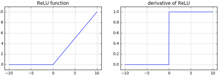
Today ReLU represents the standard for deep neural networks and has replaced functions as sigmoid and tanh.
Below are listed some of the advantages that ReLU possesses over sigmoid/tanh:
Non-vanishing gradient. During backpropagation, the function does not saturate for positive inputs, regardless of the number of layers (it can however suffer from the "dying" gradient problem, explained later). This is because the gradient of the ReLu function is always
Computationally efficient. ReLU accelerates the training speed since its derivative can be calculated by simply thresholding activations at zero, as opposed to the more computationally expensive derivative calculation of sigmoid/tanh (e.g. calculate exponentials). This is particularly relevant when designing deep neural networks.
Highly sparse neural nets. When the input for ReLU is less than or equal to
These advantages make ReLU the most used activation function today.
Nevertheless, ReLU holds some disadvantages in that neurons can “die”
during training: a large gradient can cause a ReLU neuron to update the
weights in such a way that it will always output
Softmax
The softmax function is used at the final layer of a multi-class
NN
(Goodfellow et al., 2016, pp. 180–184). It takes in an un-normalised vector and normalises it into a probability distribution;
that is, it squashes a neuron’s output
TIP
Before continuing, it is useful to understand the concept of feature vector. Check the glossary for a definition.
Training a Neural Network
The human brain is thought to gain experience modifying the strength of its inter-neuron connections. Similarly to this model, an artificial neural network gains "experience" through a training process that aims to adjust the neurons’ weights, until a desired design objective is reached (Haykin, 1994, pp. 139–141). For instance, in the case of Image Classification the objective is to correctly predict the class of a given input image.
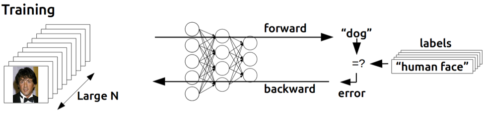
Once a NN architecture is defined, the training process can start (see Figure 5). Below are summarised the steps involved:
Initialisation. Initialise the weights and biases to certain values.
Forward propagation. The input traverses all layers of the NN and a class score is output.
Loss function. The inconsistency between the predicted class and true class is measured.
Backward propagation. The gradient of the loss function with respect to the network’s weights is calculated; this is then backpropagated to correct the weights.
Repeat steps 2 to 4. The steps 2 to 4 are repeated until the cost function is sufficiently minimised.
The next sections describe these steps in more detail.
Weight Initialisation
Correctly initialising the weights of a NN is a crucial step for training, since, especially in deep networks, bad initialisation can cause learning to halt due to the gradient’s instability.
A popular choice is to initialise the network with
random weights drawn from zero-mean Gaussian distributions (Krizhevsky
et al., 2012), however, using fixed standard deviations (e.g. 0.01)
deeper networks (e.g. more than 8 conv layers) have difficulties to
converge, as reported by Simonyan & Zisserman (2014). As discussed in
He et al. (2015), if the network uses ReLU units a better approach is
to use random weight initialisation with a standard deviation of
Transfer Learning
In some cases, it is unfeasible to train a model from scratch. This can be, for example, if the available dataset is not of a sufficient size to achieve good results, or if the training process takes too long due to the high number of parameters that need to be adjusted.
This problem can be overcome thanks to a technique called "transfer learning" (also known as "pre-training" or "fine tuning"; Pan et al., 2010). In essence, this technique allows to initialise the network’s parameters with a pretrained model’s optimised parameters; these are often trained on large datasets and require an extremely long computational time. To note is that the dataset used by the pretrained model may well come from a different domain. For example, the pretrained model’s parameters could be tailored to recognise cars, though they could be used as initial parameters for a bus recogniser.
After initialisation, the training proceeds as usual, allowing the parameters to adapt to the different dataset with the benefit of reduced training time.
Forward Propagation
In this phase, an input is propagated forward through all the network’s
layers (Haykin, 1994, pp. 123–129). The
NN
fundamentally computes a function
The shape of the final output depends on the type of activation function used in the last layer. A common choice in Image Classification is the softmax function, which computes a probability distribution over the predicted output classes.
Loss Function
A loss function describes how close the values predicted by a network are to their corresponding true values. Since the network’s output values depend on the individual neurons’ weights and biases, the aim is to apply changes to these parameters that will minimise the cost (also knows as error; Haykin, 1994).
For example, in case the softmax function is used in the final layer, the loss is
measured with the cross-entropy error function. Given the input
For a multi-class, multi-neuron neural network, the cost
Backpropagation
As mentioned in the previous section, "learning" essentially refers to
adjusting the weights and the biases of the network (i.e. its parameters) to minimise the
cost; this means that for each input vector, the output vector produced
by the network should be the same as the true output vector, or,
practically, sufficiently close to it (Rumelhart et al., 1986). In classification, this means that given an image encoding
Backpropagation (short for backward propagation of errors) is today the most popular learning procedure to adjust a network’s weights. It is based on the repeated application of the chain rule of derivatives, used to compute the influence that each weight has on the final prediction with respect to an arbitrary cost function (Riedmiller & Braun, 1993). This is shown in Figure 6.
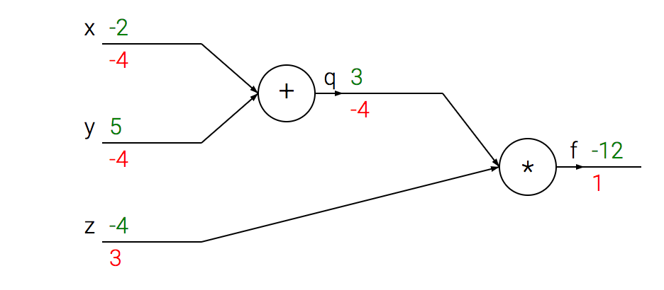
Once the partial derivatives of all weights are known, the gradient descent (GD) optimisation algorithm is used to find the global/local minima of the cost function.
The "learning rate" sets the step size of GD, which affects the time needed to reach the local/global minimum (i.e. the time for GD to converge). Choosing the right learning rate is a key operation to train a network in a time effective way. A high learning rate can approach the minimum faster but could lead to oscillation, preventing the error to fall below a certain value; a low learning rate is more precise but could be too slow to be feasible.
Due to computational limitations, often in practice only a local minimum is ever reached, as opposed to the global minimum. However, as stated by LeCun et al. (2015), poor local minima are rarely a problem in deep networks since often the system reaches solutions of very similar quality.
Final Considerations
Neural networks have experienced extreme popularity throughout history. Initially inspired by the human brain, they have come a long way since their first mathematical model in 1958. Today, however, the classic model of neural networks, the fully-connected NN, faces some key limitations. Due to its high number of parameters, it has long been deemed computationally too expensive to be useful in practical settings.
More recently, a different type of network have been proposed to overcome some of the classic NN limitations. Although briefly mentioned before, the next sections describe in more detail the architecture of Convolutional Neural Networks, which today power many of the state-of-the-art implementations found in production.
References
- Haykin, S. (1994). Neural networks: A comprehensive foundation. Prentice Hall PTR.
- Standford University. (2017). Stanford university cs231n: Convolutional neural networks for visual recognition. CNN Notes.
- McCulloch, W. S., & Pitts, W. (1943). A logical calculus of the ideas immanent in nervous activity. The Bulletin of Mathematical Biophysics, 5(4), 115–133.
- Rosenblatt, F. (1958). The perceptron: A probabilistic model for information storage and organization in the brain. Psychological Review, 65(6), 386.
- Werbos, P. (1974). Beyond regression:" New tools for prediction and analysis in the behavioral sciences. Ph. D. Dissertation, Harvard University.
- Parker, D. B. (1985). Learning logic. Center for Computational Research in Economics; Management Science. MIT Cambridge.
- Rumelhart, D. E., Hinton, G. E., & Williams, R. J. (1985). Learning internal representations by error propagation. California Univ San Diego La Jolla Inst for Cognitive Science.
- He, K., Zhang, X., Ren, S., & Sun, J. (2015). Delving deep into rectifiers: Surpassing human-level performance on imagenet classification. Proceedings of the ieee international conference on computer vision, 1026–1034.
- Changhau, I. (2017). Activation functions in neural networks.
- Xu, B., Wang, N., Chen, T., & Li, M. (2015). Empirical evaluation of rectified activations in convolutional network. CoRR, abs/1505.00853. Retrieved from http://arxiv.org/abs/1505.00853
- Krizhevsky, A., Sutskever, I., & Hinton, G. E. (2012). Imagenet classification with deep convolutional neural networks. Advances in neural information processing systems, 1097–1105.
- Glorot, X., Bordes, A., & Bengio, Y. (2011). Deep sparse rectifier neural networks. Proceedings of the fourteenth international conference on artificial intelligence and statistics, 315–323.
- Goodfellow, I., Bengio, Y., & Courville, A. (2016). Deep learning. MIT Press.
- Nazrul, M., Ishlam Patoary, M. N., Tropper, C., Lin, Z., Mcdougal, R., & Lytton, W.(2014). Neuron time warp. Proceedings - Winter Simulation Conference, 2015.
- NVIDIA. (2015). Inference: The next step in gpu-accelerated deep learning.
- Simonyan, K., & Zisserman, A. (2014). Very deep convolutional networks for large-scale image recognition. arXiv Preprint arXiv:1409.1556.
- Pan, S. J., Yang, Q., & others. (2010). A survey on transfer learning. IEEE Transactions on Knowledge and Data Engineering, 22(10), 1345–1359.
- Rumelhart, D. E., Hinton, G. E., & Williams, R. J. (1985). Learning internal representations by error propagation. California Univ San Diego La Jolla Inst for Cognitive Science.
- Rumelhart, D. E., Hinton, G. E., & Williams, R. J. (1986). Learning representations by back-propagating errors. Nature, 323(6088), 533.
- Riedmiller, M., & Braun, H. (1993). A direct adaptive method for faster backpropagation learning: The rprop algorithm. Neural networks, 1993., ieee international conference on, 586–591. IEEE.
- LeCun, Y., Bengio, Y., & Hinton, G. (2015). Deep learning. Nature, 521(7553), 436.