One-Shot Learning
Introduction
Humans have the capability to quickly learn a large number of novel objects per day. In fact, humans recognise more than 10,000 visual categories by the time they are six (Biederman, 1987, pp. 115–147).
There are an approximate 3,000 basic-level identifiable, unique and distinct concrete nouns in the English lexicon, such as "dog" and "chair" (Biederman, 1987, p. 127). Once a basic-level object is learnt, it is easy for a human to use priori knowledge of object categories to recognise new objects belonging to the same category, such as recognising that a never before seen Pug belongs to the dog category. For the same principle, humans are also extremely precise at recognising something that does not belong to the same category of a newly seen object, such as distinguish a never before seen fox to a dog. This situation is described in the literature as one-shot learning.
One-shot learning tries to emulate the human brain capability to learn new objects from a single example. The key insight for one-shot learning is that, rather than learning a new object from scratch, one can take advantage of knowledge coming from previously learned categories, no matter how different these categories might be (Li et al., 2006).
Example One-Shot Learning
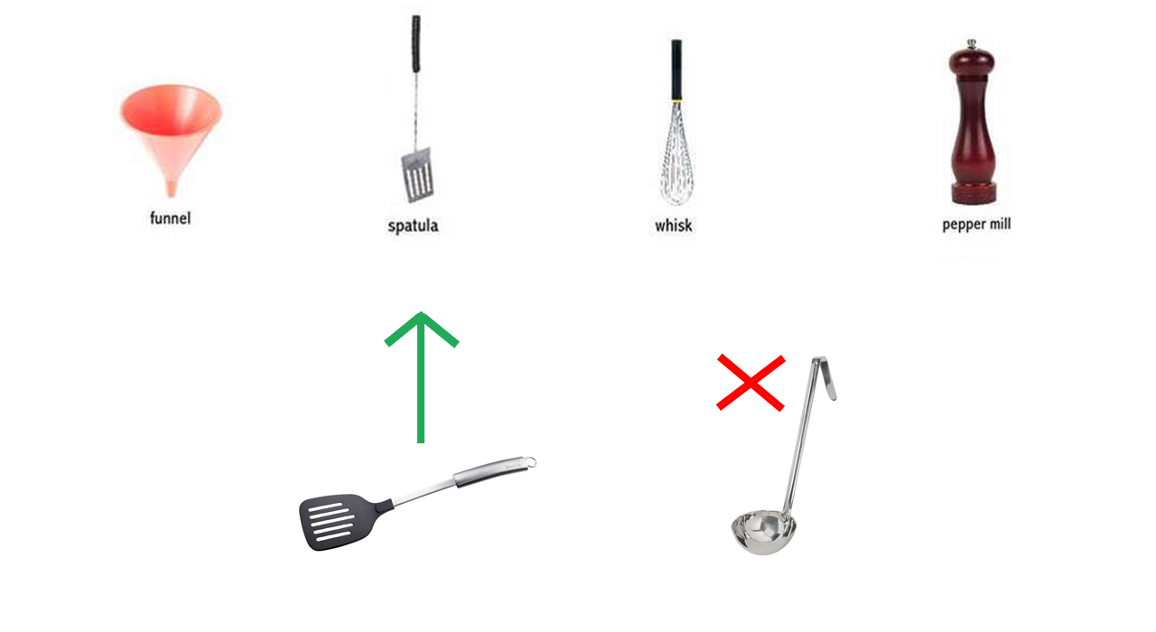
A practical example of one-shot learning is provided below. This example sees a small dataset composed of only four pictures of objects commonly found in a kitchen: a funnel, a spatula, a whisk and a pepper mill. Despite having seen only one picture for each object, when a new picture of a spatula is analysed, the system should be able to recognise it. In contrast, if it sees a picture of a ladle, then it should recognise that it is not one of the objects present in the dataset (see Figure 1).
An approach to tackle this problem involves the use of a "similarity" function, that is defined as:
where
The user can specify a certain threshold value
At recognition time, the function
What explained allows to solve the one-shot learning problem: as long as
the function
Siamese Neural Network
One of the proposed solutions to solve the one-shot learning problem involves the use of a Siamese Neural Network, which was originally introduced by Bromley and LeCun (1994) as part of a signature verification system.
The general idea is that a Siamese Network can take two images as input and output the probability that they share the same class. As outlined by Koch et al. (2015), large Siamese Convolutional Neural Networks:
Are able to make predictions about unknown class distributions even when very few examples from these new distributions are available.
Are easily trained using standard optimisation techniques.
Provide a competitive approach that does not rely upon domain-specific knowledge by instead exploiting deep learning techniques.
Architecture
The Siamese Neural Network architecture consists of two identical sub-networks joined at their outputs. The two sub-networks are constrained to have the same set of weights and parameters. At training time the two sub-networks extract features from two inputs, while a joining neuron measures the distance between the two resulting feature vectors.
This approach has two key properties:
The network ensures consistency. Weight tying guarantees that two similar images cannot be mapped by their respective sub-networks to very different locations in the feature space as each network computes the same function (Koch et al., 2015).
The network is symmetric. An image will be re-represented as the same encoding regardless of the sub-network processing it. The degree of similarity between the two images is calculated as the norm of the difference between the two image encodings. This implies that the distance between two image encodings is the same regardless of which one of the sub-networks each image is processed by.
Example of a Siamese Neural Network
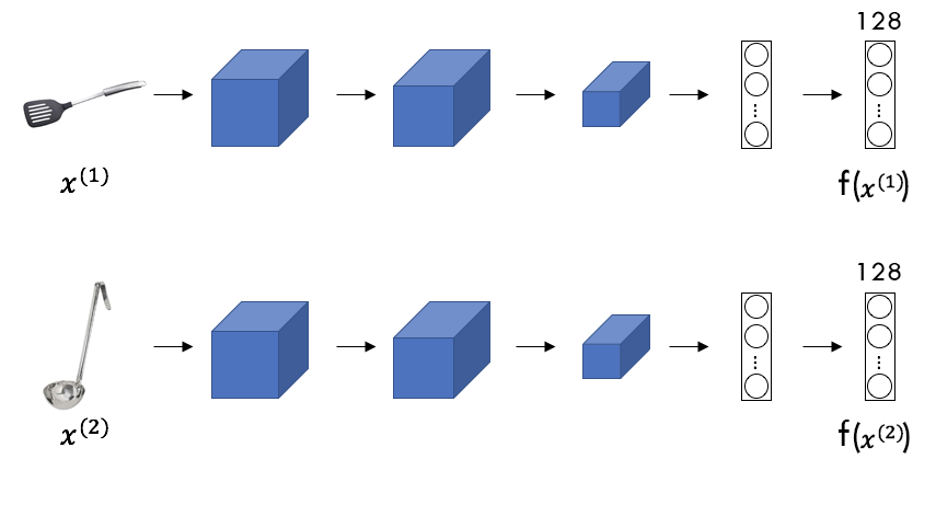
Considering two test images
The degree of difference
The objective is for the Siamese Network to learn parameters so that:
If the parameters of the
NN’s
layers are varied, different encodings are calculated for the images
Triplet Loss
A loss function measures the distance between the expected result and the result produced by a NN, that is the magnitude of error the NN made on its prediction. One way to learn the parameters of the NN so that it produces a good encoding for an input image is to define and apply a triplet-based gradient descent.
Triplet loss has gained popularity since its recent employment in Google’s FaceNet (Schroff et al., 2015), where a new approach to train face embeddings using online triplet mining is discussed.
The triplet loss takes into consideration three example images at a time: an anchor, a positive and a negative example (hence the name "triplet"). The anchor represents the base image, the positive image depicts the same object contained in the anchor and the negative depicts an object different from the one contained in the anchor. Since the positive example depicts the same object contained in the anchor, the difference between their encodings ought to be small, whereas the difference between the encodings of the anchor and the negative example ought to be large.
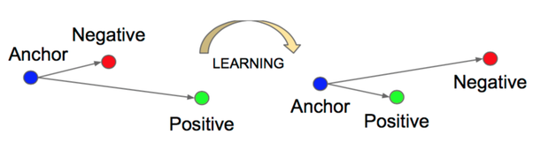
More specifically, the aim of the triplet loss function is to find some parameters for the considered NN so that the squared distance between the encodings of the anchor and the positive image is smaller than the squared distance between the encodings of the anchor and the negative image. Figure 3 illustrates the outcome that the triplet loss function strives to achieve.
Indicating with
However, to prevent the
NN
to return trivial solutions to satisfy the equation shown above, such as
outputting 0 for all the image encodings or outputting the same
encodings for the positive and negative images, it is useful to
introduce a margin
Where
To increase the effectiveness of the learning algorithm used in the
NN,
it is necessary to choose triplets that are "hard" to train on, which
means selecting images such that the value of
Considerations
Siamese CNNs have found use in variety of contexts during the past years. For example, Koch et al. (2015) use this architecture for image classification on the Omniglot dataset (Lake et al., 2015), achieving 92% accuracy in the 20-way one-shot task; Taigman et al. (2014) use it for face verification within their DeepFace system, achieving 96.17% accuracy; and Melekhov et al. (2016) use it to perform scene image classification, achieving accuracy above 80% on the shown landmarks. Despite their discrete success, however, they have not sparked particular interest in the research community.
For example, only a few attempts were made at using Siamese Networks to recognise objects (in the literal sense), although these achieved overall good results, as outlined by researchers Choy et al. (2016) and Vinyals et al. (2016). Object recognition with siamese CNNs is an interesting area that is worth researching more and could bring a definitive solution to the one-shot learning problem.
K-Nearest Neighbour
k-nearest neighbour is one of the simplest data classification algorithms, widely used when little or no prior knowledge about the distribution of the data is available. It attempts to determine what class a data point belongs to by examining the data points nearest to it. This process can be summarised in the three steps below:
Calculate the distances between a point
Pick
Find the most common class among the k-nearest points (majority voting) to calculate the class of the point
In Image Classification, an image can be re-represented as a vector
where each point in the feature space (i.e. pixel) is described as a
pair of coordinates and has a colour value associated with it. To
calculate the distance (i.e. similarity) between two image vectors
k-nearest neighbour does not require to generate a model of the dataset (i.e. no training is needed) and allows to incorporate previously unseen classes. Although k-nearest neighbour does not yield highly accurate results, it is considered a good "baseline" algorithm to which compare other one-shot learning algorithms.
According to Koch et al. (2015), 1-nearest neighbour achieves 21.7% accuracy in the 20-way one-shot classification task on the Omniglot dataset. Even though this is not as accurate as other algorithms, it is four times more accurate than random guessing, which corresponds to 5% accuracy.
Matching Networks for One-Shot Learning
The k-nearest neighbour algorithm does not require parameter optimisation, however, its performance depends on the chosen metric (e.g. L2 distance).
From this intuition, Vinyals et al. (2016) propose Matching Networks, a fully end-to-end differentiable nearest neighbour classifier. The authors acknowledge that non-parametric structures make it easier for NNs to "remember" and adapt to new training sets, and suggest that better results are achieved when a network is specifically trained to do one-shot learning. As a result, matching networks are both trained and tested on N-shot, K-way tasks.
The model proposed resembles siamese networks but has an asymmetric
architecture in that the encoding functions
Model Architecture
Given a support set of
Here,
In the above equation
The authors propose that the embedding function
References
- Biederman, I. (1987). Recognition-by-components: A theory of human image understanding. Psychological Review, 94(2), 115–147.
- Li, F.-F., Fergus, R., & Perona, P. (2006). One-shot learning of object categories. IEEE Transactions on Pattern Analysis and Machine Intelligence, 28(4), 594–611.
- Bromley, J., Guyon, I., LeCun, Y., Säckinger, E., & Shah, R. (1994). Signature verification using a "siamese" time delay neural network. Advances in neural information processing systems, 737–744.
- Koch, G., Zemel, R., & Salakhutdinov, R. (2015). Siamese neural networks for one-shot image recognition. ICML deep learning workshop, 2.
- Schroff, F., Kalenichenko, D., & Philbin, J. (2015). Facenet: A unified embedding for face recognition and clustering. Proceedings of the ieee conference on computer vision and pattern recognition, 815–823.
- Lake, B. M., Salakhutdinov, R., & Tenenbaum, J. B. (2015). Human-level concept learning through probabilistic program induction. Science, 350(6266), 1332–1338. https://doi.org/10.1126/science.aab3050
- Taigman, Y., Yang, M., Ranzato, M., & Wolf, L. (2014). Deepface: Closing the gap to human-level performance in face verification. Proceedings of the ieee conference on computer vision and pattern recognition, 1701–1708.
- Melekhov, I., Kannala, J., & Rahtu, E. (2016). Siamese network features for image matching. 2016 23rd international conference on pattern recognition (icpr), 378–383. https://doi.org/10.1109/ICPR.2016.7899663
- Choy, C. B., Gwak, J., Savarese, S., & Chandraker, M. (2016). Universal correspondence network. Advances in neural information processing systems, 2414–2422.
- Vinyals, O., Blundell, C., Lillicrap, T., Wierstra, D., & others. (2016). Matching networks for one shot learning. Advances in neural information processing systems, 3630–3638.